In our Open Data Series, we have shown how aggregated Physical and Game Intelligence metrics can be used to compare players and build archetypes, and we have also demonstrated the visualisation of individual actions through Dynamic Events data.

This time, we are introducing XY Tracking Data into the mix.

Tracking is the foundation on which all of our other data is built, and merging it with Dynamic Events provides almost infinite possibilities for analysis and visualisation. As a starting point, we will focus on how the combination provides full pitch and player context, allowing for static or animated visualisation of player actions and corresponding movements.

Our free release from the 2024/25 Australian A-League season includes 10 matches of Tracking and Dynamic Events data that can be merged in this way.

The matches, and their corresponding IDs, are: 

• Auckland FC 2 - 0 Newcastle (30/11/2024): 1886347
• Auckland FC 2 - 1 Wellington Phoenix (07/12/2024): 1899585
• Brisbane Roar 0 - 1 Perth Glory (21/12/2024): 1925299
• Central Coast Mariners 1 - 1 Melbourne City (31/12/2024): 1953632
• Sydney FC 4 - 1 Adelaide United (01/02/2025): 1996435
• Melbourne City 2 - 0 Macarthur FC (07/03/2025): 2006229
• Wellington Phoenix 2 - 3 Melbourne Victory (12/04/2025): 2011166
• Western United 1 - 0 Sydney FC (27/04/2025): 2013725
• Western United 4 - 2 Auckland FC (03/05/2025): 2015213
• Melbourne Victory 0 - 1 Auckland FC (17/05/2025): 2017461

Follow along with the code below to find out how to combine, manipulate and visualise the two datasets.

0 - Install Libraries

Before anything else, we need to install and import the necessary libraries and set our colour palette for the visualisations.

# Install libraries
!pip install numpy pandas mplsoccer skillcorner skillcornerviz

import os
from io import BytesIO
import pandas as pd
import json
import numpy as np
import requests

# Setup pitch and plot
from mplsoccer import Pitch ,VerticalPitch

#Set colour palette for viz
default_palette=[
   "#252525",
   "#00a82f", #  Green
   "#32fe6b", #  Lime
   "#7acbff", #  Pastel azure
   "#2388c8", #  Azure
   "#064c62"  #  Dark Azure
]

Now we are ready to get started.

1 - Load Tracking Data

Our first step is to load in the Tracking file for a given match. 

We will take the 30/11/2024 encounter between Auckland City and Newcastle as our example here, but you can easily select another encounter by inputting the relevant match_id (detailed in the list above) where indicated in the code.

# Use match_id to identify correct file | Default: Auckland FC 2 - 0 Newcastle (30/11/2024)
match_id = 1886347

# URL for the Tracking data file, automatically updated in line with the stipulated match_id
url = f"https://github.com/SkillCorner/opendata/raw/refs/heads/master/data/matches/{match_id}/{match_id}_tracking_extrapolated.jsonl"

raw_data=pd.read_json(url,lines=True)

raw_df = pd.json_normalize(
   raw_data.to_dict("records"),
   "player_data",
   ["frame", "timestamp", "period", "possession", "ball_data"],
)

# Extract 'player_id' and 'group from the 'possession' dictionary
raw_df["possession_player_id"] = raw_df["possession"].apply(
   lambda x: x.get("player_id")
)
raw_df["possession_group"] = raw_df["possession"].apply(lambda x: x.get("group"))

# Expand the ball_data with json_normalize
raw_df[["ball_x", "ball_y", "ball_z", "is_detected_ball"]] = pd.json_normalize(
   raw_df.ball_data
)

# Add the match_id identifier to your dataframe
raw_df["match_id"] = match_id
tracking_df = raw_df.copy()
tracking_df.head()

That final line of code will produce a list of the first few rows of the dataframe to check that the output looks correct and that we have successfully imported the Tracking data.

2 - Load Match Metadata

Next, we need to load in the metadata for our chosen match and create a dataframe with the details of all the players involved and which end their team was attacking in each half.

#match_id persists from previous code block, but you can modify or set here if running separately
#match_id = 1886347

#Set Metadata file URL
metadata_url=f"https://raw.githubusercontent.com/SkillCorner/opendata/refs/heads/master/data/matches/{match_id}/{match_id}_match.json"

response = requests.get(metadata_url)
raw_match_data = response.json()

# The output has nested json elements. We process them
raw_match_df = pd.json_normalize(raw_match_data, max_level=2)
raw_match_df["home_team_side"] = raw_match_df["home_team_side"].astype(str)


#Create a players dataframe
players_df = pd.json_normalize(
   raw_match_df.to_dict("records"),
   record_path="players",
   meta=[
       "home_team_score",
       "away_team_score",
       "date_time",
       "home_team_side",
       "home_team.name",
       "home_team.id",
       "away_team.name",
       "away_team.id",
   ],  # data we keep
)

#Establish function to convert time into seconds
def time_to_seconds(time_str):
   if time_str is None:
       return 90 * 60  # 120 minutes = 7200 seconds
   h, m, s = map(int, time_str.split(':'))
   return h * 3600 + m * 60 + s

# Take only players who played and create their total time
players_df = players_df[
   ~((players_df.start_time.isna()) & (players_df.end_time.isna()))
]
players_df["total_time"] = players_df["end_time"].apply(time_to_seconds) - players_df[
   "start_time"
].apply(time_to_seconds)

# Create a flag for the GK
players_df["is_gk"] = players_df["player_role.acronym"] == "GK"

# Add a match name
players_df["match_name"] = (
   players_df["home_team.name"] + " vs " + players_df["away_team.name"]
)

# Add a flag if the given player is home or away
players_df["home_away_player"] = np.where(
   players_df.team_id == players_df["home_team.id"], "Home", "Away"
)

# Create flag from player
players_df["team_name"] = np.where(
   players_df.team_id == players_df["home_team.id"],
   players_df["home_team.name"],
   players_df["away_team.name"],
)

# Figure out sides
players_df[["home_team_side_1st_half", "home_team_side_2nd_half"]] = (
   players_df["home_team_side"]
   .astype(str)
   .str.strip("[]")
   .str.replace("'", "")
   .str.split(", ", expand=True)
)

# Clean up sides
players_df["direction_player_1st_half"] = np.where(
   players_df.home_away_player == "Home",
   players_df.home_team_side_1st_half,
   players_df.home_team_side_2nd_half,
)
players_df["direction_player_2nd_half"] = np.where(
   players_df.home_away_player == "Home",
   players_df.home_team_side_2nd_half,
   players_df.home_team_side_1st_half,
)

# Clean up and keep the columns we need for the analysis
columns_to_keep = [
   "start_time",
   "end_time",
   "match_name",
   "date_time",
   "home_team.name",
   "away_team.name",
   "id",
   "short_name",
   "number",
   "team_id",
   "team_name",
   "player_role.position_group",
   "total_time",
   "player_role.name",
   "player_role.acronym",
   "is_gk",
   "direction_player_1st_half",
   "direction_player_2nd_half",
   "home_away_player"
]
players_df = players_df[columns_to_keep]
players_df.head()

Again, the final line produces a list of the first few rows of the dataframe to check the output.

3 - Merge Tracking and Metadata

Next, we combine the Tracking dataframe with the relevant information from the Metadata one, and adjust coordinates for in and out of possession and the two halves of play.

# 1. Merge tracking and player metadata
temp_df = tracking_df.merge(players_df, left_on="player_id", right_on="id")

# 2. Assign direction based on the current period
# Uses the period as an index to pick between 1st and 2nd half columns
temp_df['current_direction'] = np.where(
   temp_df['period'] == 1,
   temp_df['direction_player_1st_half'],
   temp_df['direction_player_2nd_half']
)

# 3. Determine possession status
# We simplify the boolean check by matching the team labels
is_home_poss = (temp_df['possession_group'] == 'home team') & (temp_df['home_away_player'] == 'Home')
is_away_poss = (temp_df['possession_group'] == 'away team') & (temp_df['home_away_player'] == 'Away')
temp_df['in_possession'] = is_home_poss | is_away_poss

# 4. Create the Flip Mask
# We flip if:
# (Attacking right-to-left AND in possession) OR (Defending left-to-right AND out of possession)
flip_mask = (
   ((temp_df['current_direction'] == 'right_to_left') & temp_df['in_possession']) |
   ((temp_df['current_direction'] == 'left_to_right') & ~temp_df['in_possession'])
)

# 5. Apply coordinate inversion
# Iterating over existing columns avoids repetitive 'np.where' blocks
coords = [c for c in ['x', 'y', 'ball_x', 'ball_y'] if c in temp_df.columns]
for col in coords:
   temp_df[col] = np.where(flip_mask, -temp_df[col], temp_df[col])

enriched_tracking_data = temp_df

4 - Load Dynamic Events, Identify Desired Actions

We now load in the Dynamic Events file for our chosen match.

#match_id persists from previous code block, but you can modify or set here if running separately
#match_id = 1886347

de_match = pd.read_csv(f"https://raw.githubusercontent.com/SkillCorner/opendata/refs/heads/master/data/matches/{match_id}/{match_id}_dynamic_events.csv")

de_match.head()

Having done so, we filter down to the events we are interested in analysing. In this case, we are looking for off-ball runs where the player successfully received the ball. 

Here, we order them by the distance covered to identify runs that are likely to be interesting subjects for visualisation, but a scout or analyst would obviously apply a more developed filter depending on the specific subject of their analysis.

#Identifying the longest off-ball runs in the match
de_match[(de_match.event_type == "off_ball_run") & (de_match.received == True)][
   [
       "player_id",
       "player_name",
       "team_shortname",
       "event_id",
       "frame_start",
       "frame_end",
       "event_type",
       "event_subtype",
       "received",
       "team_id",
       "player_in_possession_id",
       "x_start",
       "y_start",
       "x_end",
       "y_end",
       "distance_covered"
   ]

].sort_values(by="distance_covered", ascending=False)

For ease, we select the longest run that was successfully served by a pass (event_id == "1_133") as the subject of our visualisations, an underlapping run by Newcastle’s Thomas Aquilina.

5 - Static Visualisation of Tracking Data

Firstly, we will produce a static visualisation of the off-ball run, displaying the trail of the run from start point (smaller circle) to finish (unbordered circle). The attacking team will be in green; the defending team in blue. The player who made the pass will be highlighted in a lighter green.

Here is the code:

#Filtering to the relevant frames the longest received run from the Dynamic Events file

specific_event = de_match[de_match.event_id == "1_133"][
   [
       "player_id",
       "frame_start",
       "frame_end",
       "event_type",
       "team_id",
       "player_in_possession_id",
       "x_start",
       "y_start",
       "x_end",
       "y_end",
   ]
]

synced = specific_event.merge(
   enriched_tracking_data,
   left_on=["frame_end"],
   right_on="frame",
   suffixes=("_event", "_tracking"),
)

synced["runner"] = synced.player_id_event == synced.player_id_tracking
synced["ball_carrier"] = synced.player_in_possession_id == synced.player_id_tracking
synced["tip"] = synced.team_id_event == synced.team_id_tracking

synced["runner"] = synced.player_id_event == synced.player_id_tracking
synced["ball_carrier"] = synced.player_in_possession_id == synced.player_id_tracking
synced["tip"] = synced.team_id_event == synced.team_id_tracking

pitch = Pitch(
   pitch_type="skillcorner",
   line_alpha=0.75,
   pitch_length=105,
   pitch_width=68,
   pitch_color="#212121",
   line_color="white",
   linewidth=1.5,
)
fig, ax = pitch.grid(figheight=8, endnote_height=0, title_height=0)

size = 300
possession_team = synced[synced.tip == True]
ax.scatter(
   possession_team["x"],
   possession_team["y"],
   c="#00A82F",
   alpha=0.95,
   s=size,
   edgecolors="white",
   linewidths=1.5,
   zorder=10,
   label="team",
)

out_of_possession_team = synced[synced.tip == False]
ax.scatter(
   out_of_possession_team["x"],
   out_of_possession_team["y"],
   c="#0288D1",
   alpha=0.95,
   s=size,
   edgecolors="white",
   linewidths=1,
   zorder=10,
   label="team",
)

runner = synced[synced.runner == True]
ax.scatter(
   runner["x"],
   runner["y"],
   c="#00A82F",
   alpha=0.95,
   s=size,
   edgecolors="#00A82F",
   linewidths=2.5,
   zorder=10,
   label="team",
)

# Running
ax.plot(
   [runner["x_start"], runner["x"]],
   [runner["y_start"], runner["y"]],
   color="#00A82F",
   linewidth=2,
   ls="--",
)

ax.scatter(
   runner["x_start"],
   runner["y_start"],
   c="#00A82F",
   alpha=0.55,
   s=size / 2,
   edgecolors="#00A82F",
   linewidths=2.5,
   zorder=10,
   label="team",
)

ball_carrier = synced[synced.ball_carrier == True]
ax.scatter(
   ball_carrier["x"],
   ball_carrier["y"],
   c="#00E676",
   alpha=0.95,
   s=size,
   edgecolors="#00E676",
   linewidths=2.5,
   zorder=10,
   label="team",
)

And here is the output:

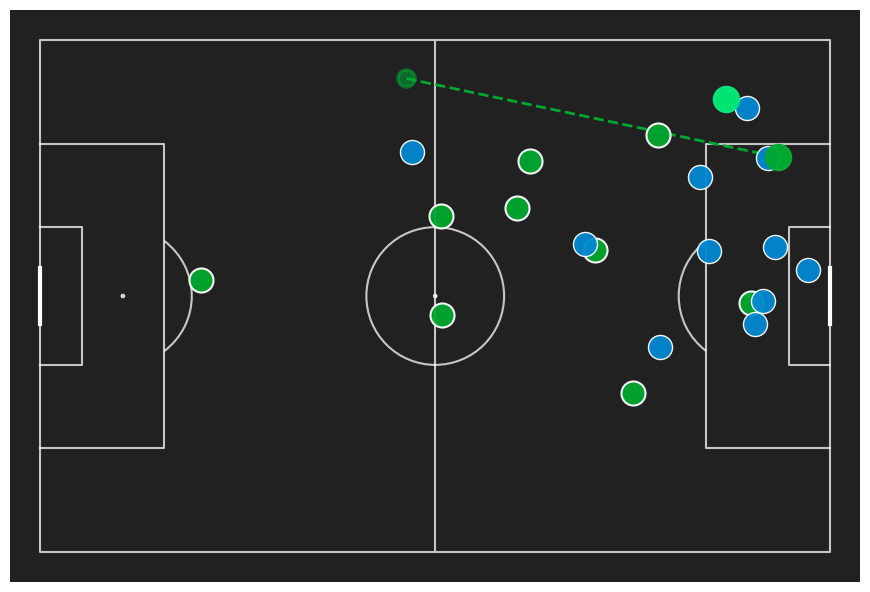
We can already see that plotting the position of all other players on the pitch at the time of the pass provides us with useful additional context over just showing the path of the run. 

And this is just a starting point. It would be relatively easy to add additional information such as player names, an average speed value or other players identified in our data as a Passing Option at the time of the pass.

6 - Animated Visualisation of Tracking Data

But to get an even fuller picture of the context, we can produce an animated visualisation of the run that shows not only its path, but the accompanying movements of all the other players – attackers and defenders alike.

We use the same visualisation cues for the ball carrier and the attacking and defending teams, and this time highlight the off-ball runner with a white border.

Here’s the code:

# Select a specific run to animate -- again we choose the same, longest received run
event_id = "1_133"
specific_event = de_match[de_match.event_id == event_id].iloc[0]

# Get frame range
start_frame = specific_event['frame_start']
end_frame = specific_event['frame_end']

# Filter tracking data
event_tracking_data = enriched_tracking_data[
   (enriched_tracking_data['frame'] >= start_frame) &
   (enriched_tracking_data['frame'] <= end_frame)
].copy()

# Sync metadata
event_tracking_data['runner'] = specific_event['player_id'] == event_tracking_data['player_id']
event_tracking_data['ball_carrier'] = specific_event['player_in_possession_id'] == event_tracking_data['player_id']
event_tracking_data['tip'] = specific_event['team_id'] == event_tracking_data['team_id']


# --- Animation Logic ---
from matplotlib.animation import FuncAnimation
from IPython.display import HTML

frames = sorted(event_tracking_data['frame'].unique())

pitch = Pitch(
   pitch_type="skillcorner",
   line_alpha=0.75,
   pitch_length=105,
   pitch_width=68,
   pitch_color=default_palette[0],
   line_color='white',
   linewidth=1.5,
)
fig, ax = pitch.grid(figheight=8, endnote_height=0, title_height=0)

# FORCE LIMITS to ensure coordinate consistency
ax.set_xlim(-52.5, 52.5)
ax.set_ylim(-34, 34)

size = 300

# Get the actual starting position from the tracking data to ensure perfect alignment
runner_start_row = event_tracking_data[(event_tracking_data['frame'] == start_frame) &
                                        (event_tracking_data['player_id'] == specific_event['player_id'])]

if not runner_start_row.empty:
   runner_start_x = runner_start_row.iloc[0]['x']
   runner_start_y = runner_start_row.iloc[0]['y']
else:
   runner_start_x = specific_event['x_start']
   runner_start_y = specific_event['y_start']


# Initialize plots
# Use consistent colors: Team in possession is always palette[1]
possession_scatter = ax.scatter([], [], c=default_palette[1], alpha=0.95, s=size, edgecolors=default_palette[1], linewidths=1.5, zorder=10, label="Team In Possession")
out_possession_scatter = ax.scatter([], [], c=default_palette[4], alpha=0.95, s=size, edgecolors=default_palette[4], linewidths=1, zorder=10, label="Team Out of Possession")
runner_scatter = ax.scatter([], [], c=default_palette[1], alpha=0.95, s=size, edgecolors="white", linewidths=2, zorder=10, label="Runner")
runner_start_scatter = ax.scatter([runner_start_x], [runner_start_y], c=default_palette[1], alpha=0.55, s=size/2, edgecolors=default_palette[1], linewidths=2, zorder=10, label="Run Origin")
runner_line, = ax.plot([], [], color=default_palette[1], linewidth=2, ls="--")
ball_carrier_scatter = ax.scatter([], [], c=default_palette[2], alpha=0.95, s=size, edgecolors=default_palette[2], linewidths=2.5, zorder=10, label="Ball Carrier")
ball_scatter = ax.scatter([], [], c="white", alpha=0.95, s=size/3, edgecolors="black", linewidths=1.5, zorder=15, label="Ball")

pitch.draw(ax=ax)

def update(frame):
   current_data = event_tracking_data[event_tracking_data['frame'] == frame]
  
   # Update positions (tracking data is now synced to match CSV)
   pos_data = current_data[current_data['tip'] == True]
   if len(pos_data) > 0:
       possession_scatter.set_offsets(pos_data[['x', 'y']].values)
   else:
       possession_scatter.set_offsets(np.empty((0, 2)))
      
   out_pos_data = current_data[current_data['tip'] == False]
   if len(out_pos_data) > 0:
       out_possession_scatter.set_offsets(out_pos_data[['x', 'y']].values)
   else:
       out_possession_scatter.set_offsets(np.empty((0, 2)))
      
   run_data = current_data[current_data['runner'] == True]
   if len(run_data) > 0:
       runner_scatter.set_offsets(run_data[['x', 'y']].values)
       # Connect start marker (CSV) to current position (Tracking)
       runner_line.set_data([runner_start_x, run_data['x'].values[0]], [runner_start_y, run_data['y'].values[0]])
   else:
       runner_scatter.set_offsets(np.empty((0, 2)))
       runner_line.set_data([], [])
      
   bc_data = current_data[current_data['ball_carrier'] == True]
   if len(bc_data) > 0:
       ball_carrier_scatter.set_offsets(bc_data[['x', 'y']].values)
   else:
       ball_carrier_scatter.set_offsets(np.empty((0, 2)))
      
   if len(current_data) > 0 and pd.notnull(current_data['ball_x'].iloc[0]):
       ball_scatter.set_offsets(np.array([[current_data['ball_x'].iloc[0], current_data['ball_y'].iloc[0]]]))
   else:
       ball_scatter.set_offsets(np.empty((0, 2)))

   return possession_scatter, out_possession_scatter, runner_scatter, runner_line, ball_carrier_scatter, ball_scatter

anim = FuncAnimation(fig, update, frames=frames, interval=100, blit=True)
import matplotlib.pyplot as plt
plt.close(fig)
print(f"Animation ready for {event_id} (Synced: {len(frames)} frames)")
HTML(anim.to_jshtml())

And here is the animated output.

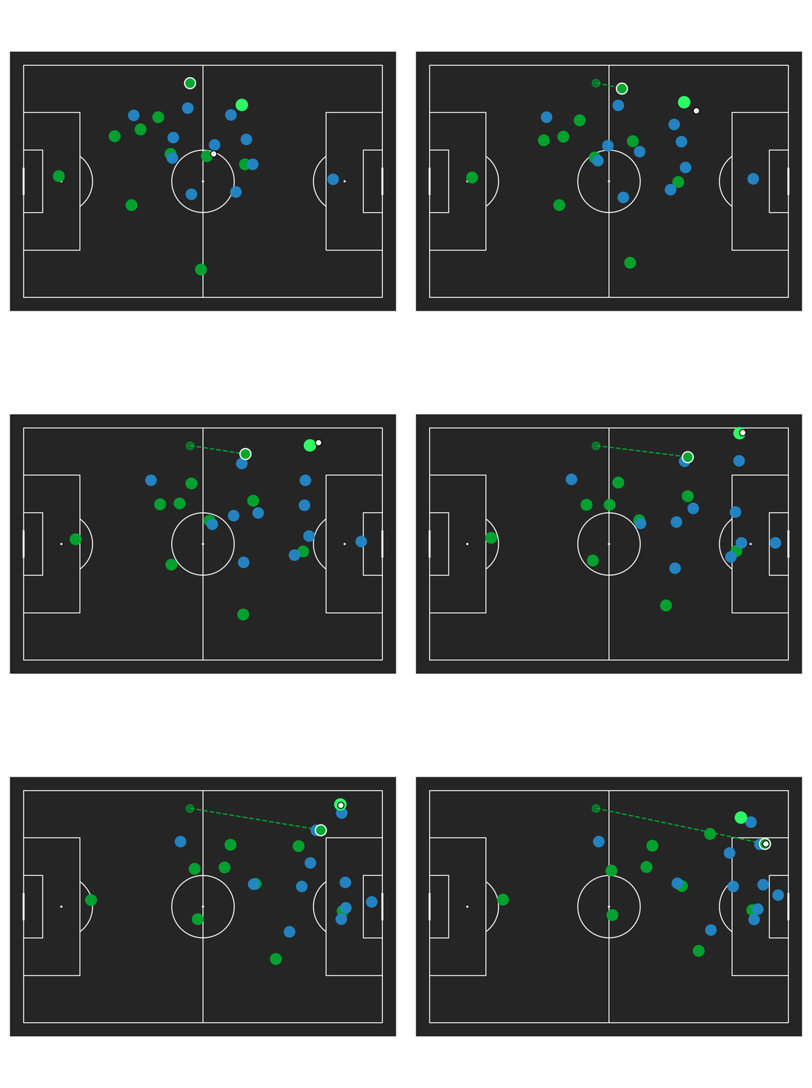
We can immediately see the value in animating the sequence to get a more complete view of the context of the run and its relationship to other players. The burst of acceleration once the underlap opportunity presents itself is clearly visible, as are the reactions of the defending team. A playlist of similar actions would at the very least provide ideas for additional avenues of investigation.

The animated visualisation can be exported to video.

#Export animation as an MP4 file

from google.colab import files
from matplotlib.animation import FFMpegWriter

#Define writer settings
writer = FFMpegWriter(fps=10, metadata=dict(artist="SkillCorner"), bitrate=1800)

#Save the animation to the Colab environment
anim.save("tracking_animation.mp4", writer=writer)

#Trigger browser download to your local machine
files.download("tracking_animation.mp4")

Or as a GIF.

#Export animation as a GIF

from matplotlib.animation import PillowWriter

#Save directly using the built-in Pillow engine
anim.save("tracking_animation.gif", writer=PillowWriter(fps=10))

files.download("tracking_animation.gif")

7 - Go Further

Fine-tuning and adding additional contextual information to either the static or animated visualisations would be an obvious continuation of the code presented here, as would shifting the focus to possession-orientated events like carries or passes, or even to particular sequences of play. For those use cases, the Dynamic Events specification provides a key framework.

But it is also worth noting that while the end goal in this case was visualisation, the ability to connect Tracking frames to Dynamic Events data opens up numerous opportunities to analyse or model spatial occupation and relationships across the pitch.

The full code for this blog is available as a Google Colab notebook for easy adaptation.

We always encourage you to share your work on social media. If you do, please reference SkillCorner as the source of the data and tag our relevant account on X/Twitter or LinkedIn.

We hope you enjoyed this part of our Open Data Series. Keep an eye on our socials for future entries.